


An understanding of wavefront optics is an important tool in the armamentarium of ophthalmologists.1-4 This concept has been used to explain and detect conditions in refractive surgery, cataract surgery, amblyopia, wound healing, keratoconus, and ocular surface abnormalities such as pterygium and dry eye.
A deeper understanding of the interpretations of wavefront optics involves the use of complex mathematics, which often prompts ophthalmologists to avoid the subject. The aim of this article is to summarize five fundamental points that can be used for a better understanding of wavefront optics. We have omitted advanced mathematics and calculus, and there is only a minimal need of basic mathematics in certain sections.
First, it is important to understand why wavefront-based assessment of refractive error is crucial in certain situations. Figure 1 shows a fictional shape that represents an eye with an irregular cornea with an approximate refractive error of -3.00 D sphere and -2.00 D cylinder, plus a little extra error (to be discussed below). Let us assume that we have access only to spherical powers (3.00, 2.00, 1.00, -1.00, -2.00, -3.00 D, etc) for correction of this error. In this scenario, our best guess fit would be the spherical equivalent, which is the spherical power plus half the cylinder power, or in this case -3 +(-2)/2= -4. So a -4.00 D sphere correction would be a sufficient compromise but not accurate enough. If we add the inventory of cylinders, we realize that the actual error is much more accurately predicted by -3.00 D sphere with the addition of -2.00 D cylinder in the correct axis.
A similar analogy between conventional refraction (retinoscopic/subjective) and wavefront-based refraction is helpful. Although we can get to a fair compromise with spherocylindrical correction, using and understanding the wavefront error of the eye helps us to measure that little extra mentioned above. This is useful in eyes in which this little extra is more than normal, such as those with pathologic corneas.
With this knowledge basis, let us dive into the world of wavefront optics.
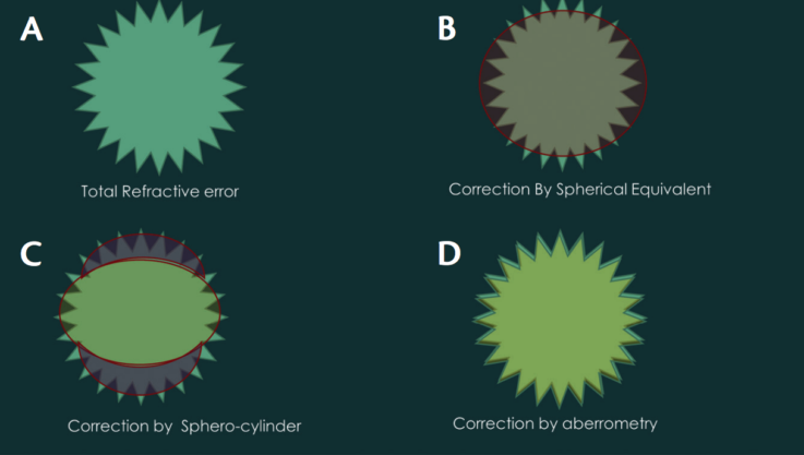
Figure 1. A fictional shape representing an eye with an irregular cornea (A) corrected by spherical equivalent (B), spherocylinder (C), and wavefront aberrometric refraction (D).

THE BASICS OF THE MATHEMATICS AND PHYSICS INVOLVED
Herein we will discuss four terms from mathematics and physics: (1) the x-y coordinate system; (2) its cousin, the polar coordinate system; (3) basic trigonometry; and (4) the wave nature of light. This is perhaps the minimum mathematics required to understand the concept of wavefront optics. However, this section can be skipped or revisited later by the reader without loss of continuity.
The Cartesian or x-y coordinate system. The x-y coordinate system is based on the old-fashioned system of walking around the block (Figure 2A). Let us take the example of Jim and Tom. When Jim says, “To get to Tom’s house from mine, walk to the signal that is 4 km from here, then take a left turn and walk 3 km to reach your destination,” Jim has essentially summarized the x-y (or the Cartesian) coordinate system. Jim’s house is the origin, the 4 km to the signal is the distance on the x-axis, and the 3 km from the signal is the distance on the y-axis. A fancier way of saying this is T(x,y) = (4,3). What if you wanted to know the actual shortest distance between Jim’s and Tom’s houses, imagining you have magical powers to fly directly but are in fuel-conservation mode? Pythagoras and his famed equation come to the rescue. Just square the two terms, add the squares, and take the square root of the sum. In this case, the result is 5 km. This can be represented mathematically as (x2 + y2)1/2. It is important to know this calculation, as it helps in understanding how wavefront terms are added and also elucidates our next topic, the polar coordinate system.
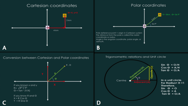
Figure 2. Basic mathematics required to understand wavefront optics, with Cartesian coor- dinates (A), polar coordinates (B), their conversion (C), and the concept of a unit circle (D).
Polar coordinate system. In principle, the polar coordinate system does the same work as the Cartesian system, ie, to locate a point. However, the origin (0,0), or Jim’s house in the previous example, is called the pole (Figure 2B). The direct distance between Jim’s and Tom’s houses that was calculated above using the Pythagorean theorem is called the radial coordinate, and the angle between the reference axis (horizontal) and the radial coordinate is called the polar coordinate, polar angle, or azimuth. The polar coordinate system makes it easier to express the Zernike polynomials (our real building blocks).
As discussed above, both of these systems, Cartesian and polar, are convertible using the Pythagorean theorem and some trigonometry (Figure 2C). Given that R and Θ (angle theta) are the radial and polar coordinates, the Cartesian coordinates will be x= R*Cosine Θ and y= R*Sin Θ. This brings us to the next points, the well-known cosine and sine.
Basic trigonometry and unit circle. In a right triangle, where one of the three angles is 90°, the longest side is the hypotenuse and the other two sides are called opposite (to our favored angle) and adjacent (Figure 2D). The sum of all angles in a triangle can only be 180°. As the angle between the opposite angle and the adjacent angle is 90°, this leaves only the remaining 90° for the other two angles. These angles interplay in a wavelike fashion, and the relationship can be given by the ratio of the sides. This is the origin of sine and cosine. Another way to visualize this fixed relationship between sine and cosine is to imagine them as two children playing on a seesaw. If one child goes up, the other comes down by a similar amount.
Finally, tangent (tan) is the ratio of the opposite and adjacent sides. In terms of Cartesian coordinates, this can be written as tan Θ = (y/x). This right triangle can be inserted into a circle, with the hypotenuse being equal to the radius. When this radius is 1 unit (cm/mm/m/any unit of distance), the circle is called a unit circle (Figure 2D). This is an important concept to understand, as Zernike polynomials are defined over a unit circle. The benefit of a unit circle is that there is no need to worry about the R from R Cosine Θ or R Sin Θ. Remember that R is the radius here, and the radius is 1. Anything multiplied by one is itself; thus, in a unit circle, the computations become generic.
Wave nature of light. Finally, we come to the physics concept, the wave nature of light. Light can be interpreted as either a wave or a particle, but, for our purpose, its wave nature is more important. All of the points that originated at the same time from a point source, such as a small light bulb (or, analogously, a pebble dropped in still water), and that are in the same state of oscillation (phase), constitute the wavefront.

UNDERSTANDING WAVEFRONT ERROR AND ITS MEASUREMENT
An ideal wavefront of light traveling through a vacuum will have no additional imperfections, as there are no refracting media to cause refraction and scattering. However, this is not the case in the real world. Atmospheric interference distorts images of the celestial bodies, and to compensate for this astronomers came up with the concept of adaptive optics. To put it briefly, deformable mirrors were used to correct these distortions. Ophthalmology borrowed the concept. In the real-world scenario, a wavefront of parallel beams of light can be distorted by the refractive error of the eye. This wavefront error can be measured by aberrometers. There are multiple principles behind these devices, but, for the sake of simplicity, we will discuss the most commonly used method: the Hartmann-Shack principle.2,4-6
Hartmann-Shack–based devices have arrays of multiple small lenses, somewhat like the compound eye of an insect, rather than a single lens as in an autorefractor or a similar device (Figure 3). These small lenses measure deviations at multiple points on different parts of the emerging wavefront. Based on the relative position of the centroids, an image of the wavefront is reconstructed and then compared with the ideal wavefront.2,4,6 This difference is the total wavefront error. It is typically measured in root-mean-square (RMS) microns and can be converted to equivalent defocus (in diopters). However, as the optical effects of 1.00 D of spherical power are not the same as those of 1.00 D of astigmatism, the equivalent effects of higher-order aberration (HOA) RMS and defocus are not same. Nonetheless, if a clinician does not want to use microns, he or she can use the following conversion formula to get the values in diopters: equivalent diopters = 4π√3 x (RMS in µm/pupil area in mm2).7

BREAKING DOWN WAVEFRONT ERROR INTO ZERNIKE POLYNOMIALS
Total wavefront error is a useful entity in itself. It gives an idea of total distortion in the eye; however, it is not of much use if we cannot break it into smaller parts. Imagine the total wavefront error to be a lump of dough. It would not make an attractive cookie at this stage. However, multiple cookie cutters can be used to shape smaller, more recognizable pieces. The benefit of using shapes such as coma, spherical aberration, and trefoil lies in the easier visualization of the data. One can break down the wavefront error into Zernike polynomials or shapes.
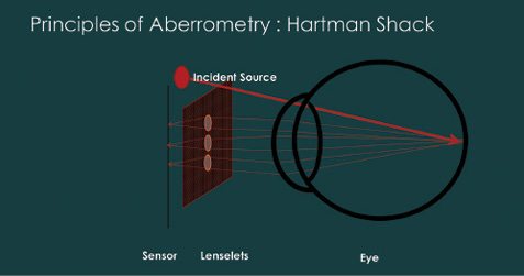
Figure 3. Schematic diagram showing the principle of Hartmann-Shack aberrometry performed on the eye.
A polynomial is an expression of two or more algebraic terms: for example, 4x2 + 3x + y. Zernike polynomials are orthogonal over a unit circle, meaning that the integral (sum) of these terms will be equal to zero. These polynomials take forms such as P3Cos3Θ (in polar coordinate form) or x3 – 3xy2 (in Cartesian format).6,8,9
The most intuitive and convenient way to write down the Zernike polynomials is the double-index scheme, Zmn. In this, the superscript index is for the meridional frequency (m), and the subscript index is of the order (n).2,6,9,10 The index n is the highest power or order of the radial polynomial (P3; therefore, 3 from the example above), and the index m describes the azimuthal frequency, or, in simpler terms, the complexity of the waveform regarding crests and troughs. For example, a meridional frequency of three in our example (3Θ) denotes three crests along the circumference of the waveform (for example, in trefoil). The polynomials with a cosine term are noted as horizontal, and the ones with a sine term are noted as vertical. Following this scheme, one can derive the common name of a polynomial from the given term.
It may seem daunting to look at Zernike polynomials at first. However, it helps to write Zernike polynomials in a visually interesting and logical way, in the form of a Zernike pyramid (Figure 4).2,6,9,10 In this scheme, the order of the polynomial increases as one moves from the apex to the base of the pyramid, and the meridional frequency changes (0, ±2, ±4 … or, ±1, ±3, ± 5 …) as one moves laterally in the pyramid. We will discuss individual aberrations in the next section. Before that, let us consider the significance of the order.
The zero order (piston) is the mean value of a wavefront or phase profile across the pupil of an optical system. The first order (tilt) aberration represents the image point location and not its quality. Thus, these do not represent or model the wavefront and are not important in our analysis of the refractive system. Our interest starts from the second order. The second-order aberrations comprise the spherocylinder and are called defocus (Z20) and astigmatism (Z2-2 and Z22). All orders larger than two are referred to as HOAs.
In a clinical scenario, most wavefront errors can be sufficiently described up to the fifth order. In distorted corneas, such as in advanced keratoconus, further expansion can be performed to include more Zernike terms, or Fourier analysis may be needed to describe the error fully.11,12 However, it should be noted that the quality of data capture in very distorted corneas is also compromised, and, therefore, the interpretation of this extra noise may be clinically distracting.

INDIVIDUAL ABERRATIONS
It is helpful to understand refractive error as a 3-D shape (Figure 5). Among the lower-order aberrations, defocus (Z20) is synonymous with spherical error. It is a symmetrical error, in that it is similar if you rotate the error along its axis. Astigmatism is described as oblique astigmatism (Z2-2) and vertical astigmatism (Z22); both are asymmetrical errors. Astigmatism has one principal meridian (axis/orientation) that corresponds to the steep shape of the 3-D refractive error.
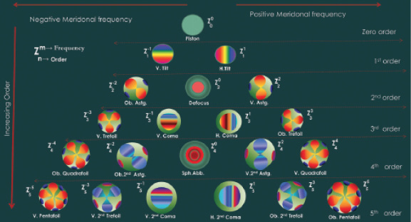
Figure 4. Schematic diagram of the Zernike pyramid.
Third-order aberration: coma (vertical Z3-1 and horizontal Z31). In coma, aberration images appear to have a tail, like a comet. Coma can be described three dimensionally as an aberration in which there is an area of more positive power and another area of more negative power in the same axis. Regarding ophthalmic optics, another way to understand coma is that it occurs when there is a difference in the power in the refracting area (cornea or lens) through which the light ray passes (in the zone of the entrance pupil). Note that this difference must be rotationally nonsymmetrical.
In ophthalmology, the most common causes for the exaggerated difference in corneal power over the pupillary area are a decentered ablation, an eccentric corneal graft, and keratoconus. In a mirror and lens system, coma occurs when the incident light rays, especially the peripheral ones, are not perpendicular to the refracting surface (Figure 6A). This can also be the case when the object plane or the image plane is not parallel to the lens plane. The visual complaint voiced by patients with coma is increased tailing around light sources (Figure 6B).
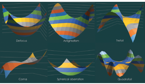
Figure 5. 3-D surface plots representing the shapes of common aberrations.
Third-order aberration: trefoil (vertical Z3-3 and oblique Z33). Trefoil means three leaves. This aberration looks like three streaks of light originating from a point source. The simplest way to understand trefoil is to look at it as astigmatism with three difference axes, or triangular astigmatism. This is evident when one looks at the 3-D image of trefoil aberration (Figure 5).
Fourth-order aberration: spherical (Z40). In a curved refracting surface, the light rays falling on the periphery tend to deviate more compared with the ones falling on the center (paraxial rays). This occurs because of the additional prismatic effect of the periphery of the curved refractive surface (Figure 7). In positive spherical aberration, peripheral rays bend more than paraxial rays and meet before the expected focus. In negative spherical aberration, peripheral rays bend less and meet beyond the expected focus. This aberration is over and above defocus, and these two should not be confused, despite their similar shapes.
The most common visual complaints of patients with increased spherical aberration are a loss of crispness and halos around images. In a normal human eye, multiple methods such as pupillary aperture and asphericity of the cornea reduce the effective spherical aberration of light entering the eye. However, certain conditions can change the spherical aberration profile of the eye. One such condition is excimer laser ablation, especially with a small optical zone and a small transition zone for a higher power (Figure 8).
Fourth-order aberration: quadrafoil. This and subsequent foils are similar to trefoil. Instead of three steep zones, qudrafoil has four, and pentafoil has five.
Secondary fourth-order aberrations: (secondary coma, secondary astigmatism, etc). These are more complex shapes based on the primary shapes described above.
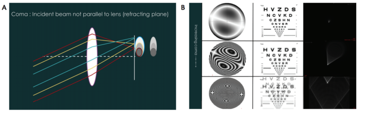
Figure 6. Optical principle of induction of coma (A). Visual simulation of coma (B). The left column shows the 2-D plots, the central column shows the simulation on a vision chart, and the right column shows the point spread function.

INTERPRETING WAVEFRONT MAPS AND CLINICAL EXAMPLES
Wavefront maps and outputs vary from device to device. The basic principles remain the same. A systematic approach can help the clinician derive the most useful data from the maps. The first thing to look for should be the quality of the scan. Some devices give an option of looking at the raw centroid image; however, most automatically decide the quality of acquisition. The next step is to look at the pupil size and the wavefront diameter. The RMS values are dependent on the pupillary diameter, and, therefore, as an attempt toward standardization, most studies report data at 4 or 6 mm for whole-eye aberrations.
Next, one should look at the total wavefront error and higher-order wavefront error. The percentage of the wavefront error governed by the HOAs can provide two important interpretations: (1) how much of the refractive error can be corrected by glasses, and (2) whether a patient’s symptoms are due to HOAs, especially in postoperative situations.
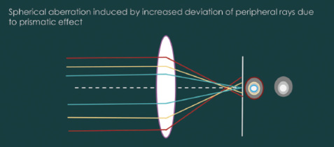
Figure 7. Optical principle of induction of spherical aberration.
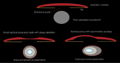
Figure 8. Schematic diagram showing clinical scenarios that can induce spherical aberration and coma. (Not drawn to scale. In real-world scenario, multiple aberrations will be induced.)
The absolute amount of total wavefront error is also useful, as it gives an overall picture of the wavefront error and the level of distortion in the eye. However, all aberrations are not equal, and different aberrations have varying effects on visual function.13,14 Thus, there is value in looking at the aberration modes separately. Individual aberrations are often demonstrated in a bar chart. Either signed or polar coefficients may be displayed, depending on the device and user selection, and one must be careful when comparing these values. A review of the aberration bar chart can give insights into the pathology, as discussed above in the sections on coma and spherical aberration.
Finally, a word about point spread function (PSF): The PSF corresponding to a specific aberration profile provides an approximation of how a point source of light (as practical examples, a distant street light or bulb) appears to a person with that particular aberration profile. It is a useful tool for understanding patient symptoms and can be used in patient counseling.
CONCLUSION
Wavefront optics involves complicated mathematics. However, understanding the basics of and rationale behind this concept can help clinicians broaden their horizons. For clinical purposes, the aforementioned principles and points are sufficiently useful for most ophthalmologists.
1. Mello GR, Rocha KM, Santhiago MR, Smadja D, Krueger RR. Applications of wavefront technology. J Cataract Refract Surg. 2012;38:1671-1683.
2. Krueger RR, Applegate RA, MacRae S. Wavefront Customized Visual Correction: The Quest for Super Vision II. Thorofare, NJ: Slack, 2004.
3. Ruttig NJ, Jancevski M, Shah SA. Evaluating wavefront analysis application in intraocular lens placement. Curr Opin Ophthalmol. 2008;19:309-313.
4. Bruce AS, Catania LJ. Clinical applications of wavefront refraction. Optom Vis Sci. 2014;91:1278-1286.
5. Platt BC, Shack R. History and principles of Shack-Hartmann wavefront sensing. J Refract Surg. 2001;17:S573-577.
6. Jagerman LS. Ophthalmologists, Meet Zernike and Fourier! Victoria, BC, Canada: Trafford, 2007.
7. Thibos LN, Himebaugh N, Coe CD. Wavefront refraction. In: Benjamin WJ, ed. Borish’s Clinical Refraction. 2nd ed. St. Louis, MO: Butterworth Heinemann Elsevier, 2006.
8. van Brug HH. Efficient Cartesian representation of Zernike polynomials in computer memory. Proc SPIE. 1997;382-392.
9. McAlinden C, McCartney M, Moore J. Mathematics of Zernike polynomials: a review. Clin Experiment Ophthalmol. 2011;39:820-827.
10. Thibos LN, Applegate RA, Schwiegerling JT, Webb R. Appendix A: Optical Society of America’s standards for reporting optical aberrations. In: Porter J, Queener HM, Lin JE, Thorn K, Awwal A, eds. Adaptive Optics for Vision Science: Principles, Practices, Design, and Applications. Hoboken, NJ: John Wiley & Sons, 2006.
11. Dai GM. Comparison of wavefront reconstructions with Zernike polynomials and Fourier transforms. J Refract Surg. 2006;22:943-948.
12. Yoon G, Pantanelli S, MacRae S. Comparison of Zernike and Fourier wavefront reconstruction algorithms in representing corneal aberration of normal and abnormal eyes. J Refract Surg. 2008;24:582-590.
13. Applegate RA, Sarver EJ, Khemsara V. Are all aberrations equal? J Refract Surg. 2002;18: S556-562.
14. Applegate RA, Ballentine C, Gross H, Sarver EJ, Sarver CA. Visual acuity as a function of Zernike mode and level of root mean square error. Optom Vis Sci. 2003;80:97-105.
Suggested further reading:
Krueger RR, Applegate RA, MacRae S. Wavefront Customized Visual Correction: The Quest for Super Vision II. Thorofare, NJ: Slack, 2004.
Jagerman LS. Ophthalmologists, Meet Zernike and Fourier! Victoria, BC, Canada: Trafford, 2007.
Vishal Jhanji, MD, FRCOphth
• Assistant Professor of Ophthalmology, The Chinese University of Hong Kong
• Honorary fellow, Centre for Eye Research Australia, University of Melbourne, Royal Victorian Eye and Ear Hospital, Australia
• vishaljhanji@cuhk.edu.hk
• Financial disclosure: None
Gaurav Prakash, MD, FRCS (Glasgow)
• Cornea and refractive surgeon, NMC Specialty Hospital, United Arab Emirates
• drgauravprakash@gmail.com
• Financial disclosure: None